From Job Ads to Forecasts: PostgreSQL, Python and Power BI

A completed job-ad analytics project: ads normalised in PostgreSQL, cleaned with Python, refreshed by scheduled AWS pipelines, reported as Power BI KPIs on one semantic model and forecast with time-series models.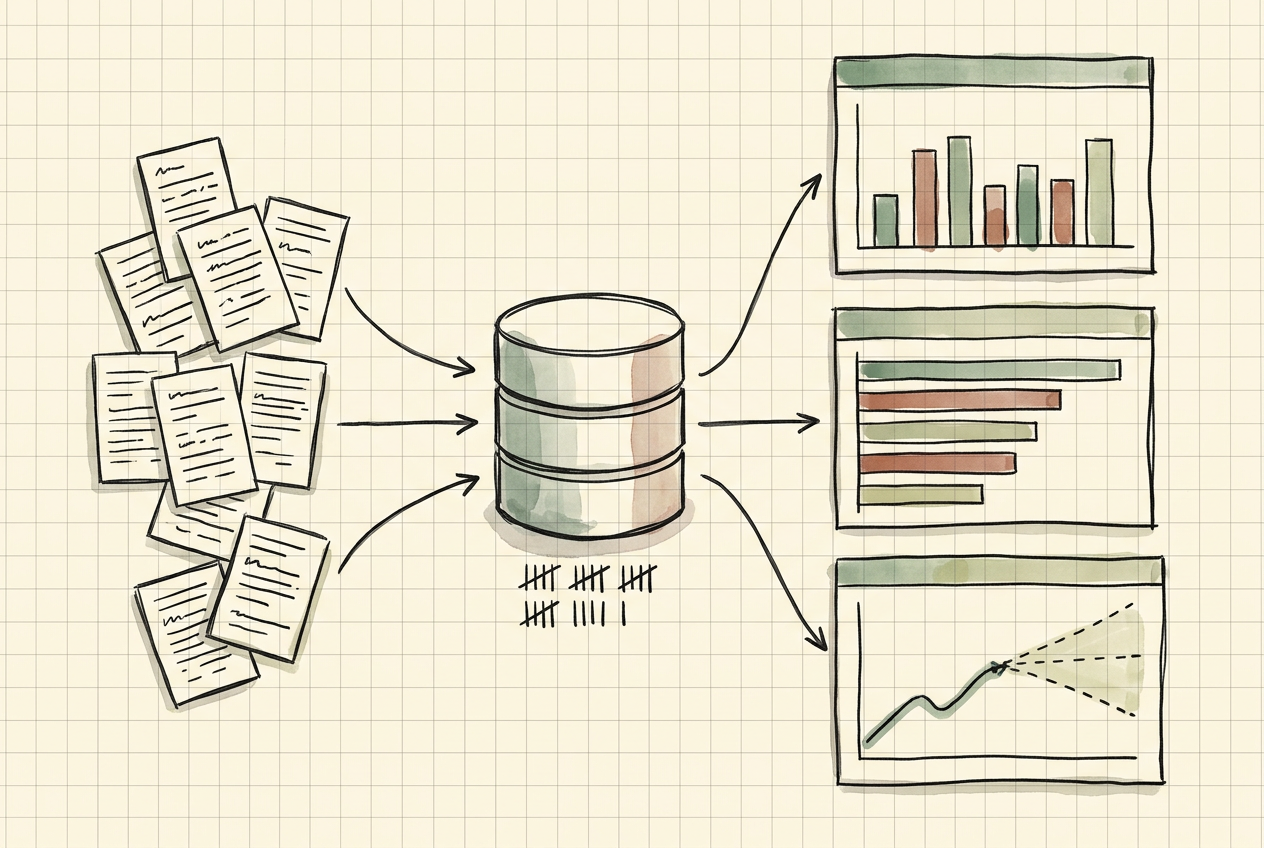

From Job Ads to Forecasts: PostgreSQL, Python and Power BI

One job ad says little: a title, a description, a location, sometimes a salary. Collected over time, ads show which roles are in demand, where that demand sits and which skills keep coming up. The client wanted to read job ads that way. Raw ad text can't be counted reliably, though. Titles are free text, locations are inconsistent and skills are buried in prose.

We built a job-ad analytics workspace for the client's analysts and business stakeholders. Ads were collected and normalised into a PostgreSQL database, then cleaned and enriched with Python. Scheduled pipelines on AWS kept the data refreshed. Power BI reports and dashboards read from one semantic model, so each KPI for demand, skills and posting activity had a single definition. Time-series forecasts built on the same history projected job-ad demand, along with revenue and sales from operational data.

Why job ads are hard to count

Job-ad data looks simple until you try to report on it. People write titles however they like, so the same role appears as "Data Analyst", "Analytics Specialist" and "Data & Reporting Analyst". Locations arrive as city names, regions, postcodes and typos. Skills sit in the description text, not in a field. The same vacancy can be posted twice, once by the employer and once by an agency. Salary is often missing, and when it is given, the format varies.

A raw row count answers none of the questions the business actually asks:

How many ads did this role family get this quarter, compared with last quarter?
Which skills are rising?
Where is demand concentrated?
Is the number of new ads likely to keep rising next quarter?

Each of those needs a stable definition, a clean table and a measure that everyone reads the same way.

What we built

We delivered one analytics path from raw ads to reported and forecast numbers:

A PostgreSQL database holding ads, employers, locations, roles and skills in related tables. SQL was used to develop the schema, analyse the data and check what had been loaded.
Python cleaning and enrichment, which turned ad text into structured fields (role family, seniority, location and mentioned skills) and flagged near-duplicate ads.
Scheduled pipelines on AWS that refreshed the database and ran checks before the reporting tables were replaced.
A Power BI semantic model with shared DAX measures, so each KPI was defined once instead of once per report.
Dynamic Power BI reports and dashboards for demand, skills and posting activity.
Predictive analytics in Python, including time-series forecasts for job-ad demand and for revenue and sales from operational data.
Agile delivery inside the client's SAFe setup, with AI-assisted analysis tools used for routine query and rule work.

How a job ad became a KPI

The ad was collected with its context. Each record kept its raw text, its publication date and a reference to where it came from, so any number could be traced back to the ads behind it.
The ad was normalised into related tables. Its employer, location, role and skills went into their own tables, linked by keys, instead of into one wide sheet.
Python read the text. Rules extracted the role family, seniority, location and mentioned skills. Near-duplicate ads were flagged before they could be counted twice.
SQL checked the load. Queries compared record counts between stages, looked for ads with missing locations and confirmed that the refresh had loaded the periods it was supposed to load. Only then were the reporting tables replaced.
The semantic model turned rows into measures. In Power BI, a KPI such as ads per role family per period existed as one DAX measure, and every visual used that measure.
Reports and dashboards showed the result. Dashboards carried the headline KPIs. The reports behind them held the detail, down to the ads that made up a number.
The same history fed the forecasts. Time-series models projected the series forward, and their output was checked against earlier periods before the business saw it.

Steps 1 to 4 ran on the AWS schedule at every refresh. Each new ad went through the same rules as every ad before it.

Database and pipelines

PostgreSQL held the analysis layer. Ads, employers, locations and skills sat in separate tables with defined keys, so a role-family trend took a join and an aggregate instead of a manual reclassification. The schema and queries used standard PostgreSQL data definition, data manipulation and query features, all covered in its documentation. SQL also did the evaluation work described in step 4, so a broken refresh was caught in the database before it reached a report.

Python handled what SQL does badly: reading ad text. Cleaning and enrichment ran as scripted jobs, so the same rules applied at every refresh. The same rules applied to every refresh, not to a hand-cleaned extract. The jobs ran on a schedule on AWS, and every run ended with the checks above.

KPIs and dashboards in Power BI

Power BI sat on top as one semantic model, not a set of separate workbooks. In Power BI, measures are formulas written in DAX. Their results recalculate as users filter and interact with a report, and a measure can be added to any visual like a normal field (Measures in Power BI). Because the KPIs lived in the model, two reports could not show two different versions of "ads this quarter".

Microsoft describes a Power BI dashboard as a single page of tiles. Tiles are pinned from reports, each report is built on a semantic model, and selecting a tile opens the report behind it (Power BI dashboards). We used that split. Dashboards showed the headline numbers, and the reports held the breakdowns.

The KPIs were organised around the questions the business kept asking:

Demand: ad volume by role family, region and seniority, compared period on period.
Skills: the most requested skills and how that ranking changed over time.
Posting activity: how many ads were new in each period and how many were duplicates of ads already counted.

Anyone could follow a surprising number down to the ads behind it and check it.

Forecasting demand and revenue

The forecasts used the same clean history. For job-ad demand, the input was the count of ads per role family over time. For revenue and sales, it was the operational figures the business already recorded. Hiring and sales both follow the calendar, so we checked for seasonality before choosing a method. A forecast that ignores the calendar can't anticipate the recurring peaks.

The forecasting models and the other predictive and machine-learning work were built in Python. Each model was tested against held-back periods before the business saw its output. Reports showed forecasts next to actuals, as a range rather than a single line.

Power BI also has a built-in forecast for line charts in its Analytics pane, with settings such as forecast length and confidence interval (Analytics pane in Power BI). Visualitics' guide compares that built-in option with models written in R or Python and run inside Power BI. It also walks through splitting history into training and validation periods (Forecasting in Power BI). That split is the same discipline we applied before any forecast reached a report.

How we worked with the client

The work ran inside the client's SAFe organisation. Analysis requests were kept as a prioritised backlog and planned with the rest of the work in each increment. SAFe describes PI Planning as a cadence-based event that aligns teams and stakeholders to shared objectives, ties development to business context and surfaces dependencies between teams (PI Planning).

That structure mattered more for definitions than for scheduling. A KPI is a shared agreement. The fastest way to reach one was to have the analyst, the owner of the number and the people who use it in the same planning conversation. AI-assisted analysis tools took on routine work, such as drafting queries and reviewing extraction rules. Their output was checked against the database before it reached a report.

Conclusion

The client ended up with a working job-ad analytics path rather than a set of one-off reports. Ads were normalised in PostgreSQL, and Python turned their text into structured fields. Refreshes ran automatically on AWS. KPIs were defined once in a Power BI semantic model, and the forecasts for demand, revenue and sales showed their uncertainty.

The path was the part that lasted. Every new ad entered the same pipeline, landed in the same tables and fed the same measures as every ad before it. Each new question about the market started from a shared definition rather than a fresh extract.